[RL Tutorial 01] An Overview of Reinforcement Learning

This is a tutorial series, written to help both myself and the reader build up a systematic knowledge framework for RL.

1. What Is Reinforcement Learning?

“When you hit a problem you cannot solve with optimization, just throw RL at it and train.” — Hung-yi Lee

In machine learning, people usually speak of three basic paradigms: supervised learning, unsupervised learning, and reinforcement learning. This taxonomy always puzzled me a little, because RL never quite seemed to fit. If supervised learning means “learning from labeled training data” and unsupervised learning means “learning from unlabeled training data,” then those two already form a perfect partition of the whole space. So why do we need RL at all? And when should we reach for it?

Why Do We Need RL?

Supervised and unsupervised learning both extract some kind of pattern from data; the only difference is whether the data carries labels. But labeled or not, both work with static data — in their world there is no such thing as an environment. Reinforcement learning, by contrast, is concerned with how to learn an optimal policy by interacting with an environment. Its data is a sequence of states, actions, and rewards produced during that interaction: it is dynamic data. Its goal is not to learn the pattern of the data, but to learn how to choose the best action in a given environment so as to maximize cumulative reward.

This is what RL can do that the others cannot: it can model dynamic problems that involve interaction with an environment.

When Should We Use RL?

Reinforcement learning generally fits scenarios that require interacting with an environment and learning an optimal policy by trial and error — robot control, games, autonomous driving, and so on.

More generally, if you can frame your problem as a sequential decision-making problem involving interaction with an environment, and you can define a suitable reward signal, then RL is worth trying. This modeling perspective is remarkably universal; a great many problems can be bent into this shape.

A certain professor known for his cheeky lecturing style once said: “When you hit a problem you cannot solve with optimization, just throw RL at it and train.” Behind the joke lies RL’s distinctive appeal: it does not need an explicit objective function. All it needs is a reward signal. Objective functions that are non-convex and painfully hard to optimize are no obstacle to RL; even a discrete parameter space is fine. Just throw RL at it and train.

Defining RL

The heart of reinforcement learning is the interaction between an agent and an environment. Guided by a reward signal, the agent grows and learns through this interaction. This closely resembles how living organisms learn — and indeed the field drew inspiration from neuroscience. If you are curious, look into the history of how Sutton invented the TD algorithm; Part 2 (Breakthrough 2) of A Brief History of Intelligence gives an accessible treatment of the topic.

With that, we can attempt a definition. Reinforcement learning (RL) is a family of algorithms for solving sequential decision-making problems. The crux of such problems is how to design an agent that, through interaction with an external environment, learns an optimal decision policy to guide its actions so as to maximize the expected cumulative reward.

During the interaction, the agent maintains an internal state \(s_t\) and selects an action \(a_t = \pi(s_t)\) according to a policy \(\pi\). Having received the action, the environment returns an observation \(o_{t+1}\), and the agent uses that observation to update its internal state via a state-update function \(s_{t+1} = U(s_t, a_t, o_{t+1})\).

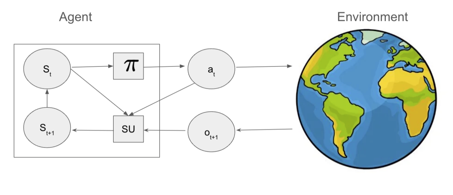
Figure: A schematic of agent-environment interaction. The agent receives observation \(o_t\) and emits action \(a_t\); the environment receives \(a_t\) and emits a new observation \(o_{t+1}\).

Before we go on, let me introduce a few core concepts. Don’t worry about memorizing them now — a rough impression is enough:

State: the situation the agent is in. In a maze game, for instance, the agent’s position is the state.
Action: an operation the agent can perform. In a maze game, the actions are “up,” “down,” “left,” and “right.”
Reward: the environment’s feedback on the agent’s behavior. In a maze game, reaching the goal yields a positive reward and bumping into a wall yields a negative one.
Policy: the rule by which the agent picks an action given the current state. In a maze game, a policy might say “if you are on the left side, move right.”
Sequential decision making: the problems RL deals with usually involve a series of decisions rather than a single one. In a maze game, every step the agent takes is a decision.
Markov process: a system whose future state depends only on the current state, not on past states. Many RL problems can be modeled as Markov decision processes (MDPs).

2. The Objective of Reinforcement Learning

Why the Mathematical Language Matters

Next we will describe RL’s objective in more precise mathematical language. Readers unfamiliar with this notation may find it intimidating, but I still recommend working until you fully understand these symbols — it will pay off later. Intuition can get you started faster, but intuition alone will not carry you far.

This tutorial introduces the notation only briefly and cannot cater to every level of background. If you run into a symbol you don’t understand, here is a trick: make full use of AI and have it explain the symbol to you. In my experience, today’s mainstream AI models are more than capable as STEM tutors. Two things are asked of you: first, be an eager student who keeps asking the right questions until it clicks; second, keep a rigorous, cross-checking attitude — AI can be wrong, so verify answers from multiple sources.

Maximizing the Expected Cumulative Reward

As we said, the goal of reinforcement learning is to find an optimal policy \(\pi^*\) that maximizes the expected cumulative reward, which can be written as:

\[V^{\pi}(s_0) = E\left[\sum_{t=0}^{T} R(s_t, a_t)\right]\]

where:

\(s_0\) is the agent’s initial state.
\(R(s_t, a_t)\) is the reward function, giving the reward obtained by taking a given action in a given state.
\(V^{\pi}(s_0)\) is the expected cumulative reward starting from initial state \(s_0\) under policy \(\pi\).
\(E\) denotes the expectation, i.e. the average cumulative reward across all possible trajectories. More precisely, the expectation is taken over the following distribution:

\[\begin{aligned} p(a_0, s_1, a_1, \ldots, a_T, s_T \mid s_0, \pi) = \; & \pi(a_0 \mid s_0) P_{\text{env}}(o_1 \mid a_0) \delta(s_1 = U(s_0, a_0, o_1)) \\ \times \; & \pi(a_1 \mid s_1) P_{\text{env}}(o_2 \mid a_1, o_1) \delta(s_2 = U(s_1, a_1, o_2)) \\ \times \; & \pi(a_2 \mid s_2) P_{\text{env}}(o_3 \mid a_{1:2}, o_{1:2}) \delta(s_3 = U(s_2, a_2, o_3)) \times \cdots \end{aligned}\]

Here \(P_{\text{env}}\) is the environment’s observation distribution (usually unknown) and \(\delta\) is the Dirac delta function.

The optimal policy \(\pi^*\) is then defined as:

\[\pi^* = \arg\max_{\pi} V^{\pi}(s_0)\]

3. A General Model of Reinforcement Learning

The Diagram

To describe reinforcement learning more clearly, we usually resort to a general model. In it, the environment is modeled as a controlled Markov process, while the agent learns through continual interaction with it. Here we borrow the diagram from Kevin Murphy’s tutorial directly:

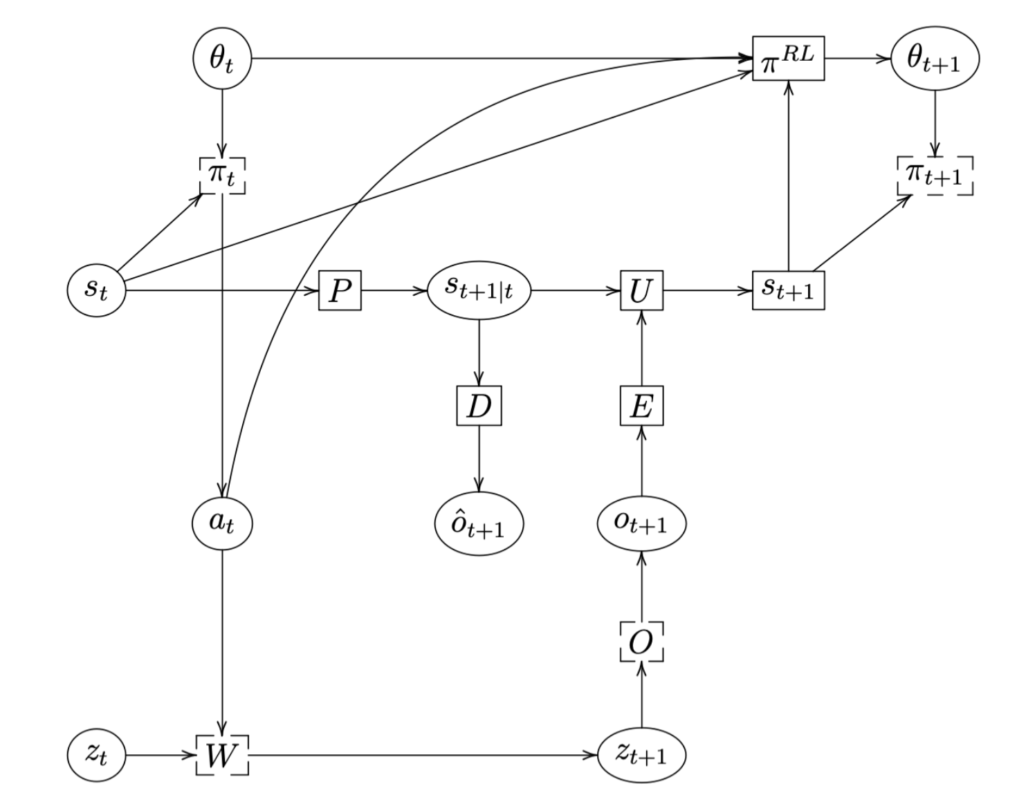
Figure: The general model of agent-environment interaction. It includes the agent’s internal state \(s_t\), prediction function \(P\), observation decoder \(D\), observation encoder \(E\), state-update function \(U\), and policy \(\pi_t\); plus the environment’s hidden state \(z_t\), world model \(W\), and observation model \(O\).

Don’t let the diagram scare you. Like the mathematical notation, once you are familiar with the pieces you will find them both simple and intuitive. Let us walk through it module by module.

The Environment Model

The environment has a hidden state \(z_t\) representing its true situation. This state is updated according to the agent’s action plus some random noise, a process captured by a transition function \(W\):

\[z_{t+1} = W(z_t, a_t, \epsilon)\]

The agent cannot observe the true state \(z_t\) directly; it only receives an observation \(o_{t+1}\) through the observation model \(O\):

\[o_{t+1} = O(z_{t+1}, \epsilon_{t+1})\]

where \(\epsilon\) is random noise.

As an aside: thanks to the AI boom set off by LLMs, you may have heard of the concept of a “world model.” A world model is simply “the external world inside the agent’s head” — it represents the agent’s understanding and prediction of its environment. In RL terms, the world model is exactly the transition function plus the reward function.

The Agent Model

The agent maintains its internal belief state \(s_t\) through a state-update function \(S_U\). This state reflects the agent’s understanding of the environment.

\[s_{t+1} = S_U(s_t, a_t, o_{t+1})\]

To describe the agent’s behavior more precisely, we can split \(S_U\) into two parts.

The prediction function \(P\) predicts the next state from the current state and action:

\[s_{t+1 \vert t} = P(s_t, a_t)\]

The update function \(U\) then refines that prediction using the observation:

\[s_{t+1} = U(s_{t+1 \vert t}, o_{t+1})\]

So \(S_U\) can be written as:

\[S_U(s_t, a_t, o_{t+1}) = U(P(s_t, a_t), o_{t+1})\]

Encoder and Decoder

These two components are actually optional, and they are what make the diagram above look more complicated than it is. When do we need them?

If the observation is high-dimensional — an image, say — we can use an encoder \(E\) to turn it into a low-dimensional embedding \(e_{t+1}\):

\[e_{t+1} = E(o_{t+1})\]

The state update then becomes:

\[s_{t+1} = U(s_{t+1 \vert t}, e_{t+1})\]

We can also use a decoder \(D\) to predict the next observation \(\hat{o}_{t+1}\):

\[\hat{o}_{t+1} = D(s_{t+1 \vert t})\]

Finally, the policy \(\pi_t\) by which the agent picks an action given the current state can be written as:

\[a_{t+1} = \pi_t(s_{t+1}) = \pi(s_{t+1}; \theta_t)\]

The policy parameters \(\theta_t\) are updated by the reinforcement learning algorithm.

Summary

Reinforcement learning has to handle three interacting stochastic processes:

The environment state \(z_t\), which is influenced by the agent’s actions.
The agent’s internal state \(s_t\), which reflects its understanding of the environment.
The policy parameters \(\theta_t\), which are updated based on that internal state.

This framework is highly general and can give rise to a wide variety of RL algorithms. We will meet them one by one in later chapters, and you can come back here to compare notes and deepen your understanding.

4. Case Study: Walking Through a Maze

To make these concepts concrete, let us look at an intuitive example: walking through a maze.

Problem Statement

Suppose we have a 5 * 5 maze in which an agent (a small robot, say) must start at \(S\) and, through a series of actions, reach the goal \(G\). The maze may contain obstacles such as walls, which the agent must avoid. The objective is to find an optimal path from \(S\) to \(G\) that maximizes cumulative reward.

Here is a sketch of the maze:

+---+---+---+---+---+
| S |   |   | W | G |
+---+---+---+---+---+
|   | W |   | W |   |
+---+---+---+---+---+
|   | W |   |   |   |
+---+---+---+---+---+
|   |   |   | W |   |
+---+---+---+---+---+
|   | W |   |   |   |
+---+---+---+---+---+

where:

S marks the start.
G marks the goal.
A blank cell is passable.
W marks a wall or obstacle and cannot be crossed.

Casting It as a Reinforcement Learning Problem

We need to model this maze as a reinforcement learning problem so that the concepts introduced earlier can be applied.

State

Here the state is simply the agent’s position in the maze. Since the maze is a 5 * 5 grid, the state space is the set of all possible grid positions:

\[\mathcal{S} = \{(x, y) \mid x, y \in \{0, 1, 2, 3, 4\}, \text{the cell is not a wall}\}\]

For example, the start \(S\) might sit at \((0, 0)\) and the goal \(G\) at \((4, 0)\). The size of the state space depends on the size of the maze and the placement of the walls.

Action

In each state the agent can choose among these actions:

Up
Down
Left
Right

so the action space is:

\[\mathcal{A} = \{\text{Up}, \text{Down}, \text{Left}, \text{Right}\}\]

Note that at the maze boundary or next to a wall, some actions may be infeasible. If the agent is in the leftmost column, for instance, it cannot move left.

Reward

The design of the reward function is crucial in reinforcement learning. To encourage the agent to find the shortest path, we can design the rewards as follows:

Each step taken earns a negative reward of -1. This makes every step costly and encourages the agent to reach the goal quickly.
Bumping into a wall or attempting an infeasible action (such as stepping outside the maze) earns a larger negative reward of -5, strongly penalizing such behavior.
Reaching the goal \(G\) earns a sizeable positive reward of 10, encouraging the agent to complete the task.

A reward design like this steers the agent toward a path through the maze that is both fast and safe.

Policy

The policy, written \(\pi(s)\), is the rule by which the agent chooses an action in each state. Our goal is to learn an optimal policy \(\pi^*\) that maximizes the expected cumulative reward from any starting state.

Objective

The agent’s objective is to find a path from start \(S\) to goal \(G\) that maximizes the expected cumulative reward. Because every step incurs a negative reward, a larger cumulative reward means fewer steps taken and a better path.

Agent-Environment Interaction

In this maze example, the interaction between agent and environment proceeds as follows:

Initial state: the agent stands at the start \(S\), denoted state \(s_0\).
Observe the state: the agent perceives its current position.
Choose an action: following the current policy \(\pi(s_t)\), it selects an action \(a_t\).
Execute the action: the agent attempts to move to the next position.
Receive a reward: based on the outcome of the move, the environment hands the agent the corresponding reward \(R(s_t, a_t)\).
Enter the next state: the agent updates its current position to the new state \(s_{t+1}\).
Update the policy: using the reward received and the new state, the agent adjusts its policy (this step belongs to the learning algorithm).
Repeat: until the agent reaches the goal \(G\) or hits the step limit.

5. Implementation

Below is a concrete implementation that gives the reader an environment to play with directly. We use OpenAI’s Gym library to build the environment and train the agent to find the optimal path with the Q-Learning algorithm. For now you need not understand how to use Gym, nor how Q-Learning works — it is enough to follow the logic roughly and get it running in your own environment.

1. Install the Required Libraries

First, make sure OpenAI Gym and the other dependencies are installed:

pip install gym
pip install numpy
pip install matplotlib

2. Define the Maze Environment

We create a custom maze environment inheriting from gym.Env and implement the necessary methods.

import gym
from gym import spaces
import numpy as np

class MazeEnv(gym.Env):
    """
    A custom maze environment inheriting from gym.Env
    """
    metadata = {'render.modes': ['human']}

    def __init__(self):
        super(MazeEnv, self).__init__()
        # Define the action space and the state space
        # Action space: up, down, left, right
        self.action_space = spaces.Discrete(4)

        # State space: the agent's position in the maze (2D coordinates)
        self.maze_size = (5, 5)
        self.observation_space = spaces.Box(low=0, high=4, shape=(2,), dtype=np.int32)

        # Define the maze (0 is open ground, -1 is a wall)
        self.maze = np.zeros(self.maze_size)
        self.maze[0, 3] = -1  # wall positions
        self.maze[1, 1] = -1
        self.maze[1, 3] = -1
        self.maze[2, 1] = -1
        self.maze[3, 3] = -1
        self.maze[4, 1] = -1

        # Start and goal
        self.start_pos = (0, 0)
        self.goal_pos = (0, 4)

        # The agent's initial position
        self.agent_pos = self.start_pos

    def step(self, action):
        """
        Execute an action
        """
        # Map each action to a movement
        directions = {
            0: (-1, 0),  # up
            1: (1, 0),   # down
            2: (0, -1),  # left
            3: (0, 1)    # right
        }

        # Compute the new position from the action
        move = directions[action]
        new_pos = (self.agent_pos[0] + move[0], self.agent_pos[1] + move[1])

        # Check whether the new position lies inside the maze
        if (0 <= new_pos[0] < self.maze_size[0]) and (0 <= new_pos[1] < self.maze_size[1]):
            # Check whether the new position is a wall
            if self.maze[new_pos] != -1:
                self.agent_pos = new_pos  # update the position
                reward = -1  # negative reward for each move
                done = False
            else:
                # Bumped into a wall
                reward = -5  # penalty for hitting a wall
                done = False
        else:
            # Stepped outside the maze
            reward = -5  # penalty for going out of bounds
            done = False

        # Check whether the goal has been reached
        if self.agent_pos == self.goal_pos:
            reward = 10  # positive reward for reaching the goal
            done = True

        obs = np.array(self.agent_pos)
        info = {}
        return obs, reward, done, info

    def reset(self):
        """
        Reset the environment to its initial state
        """
        self.agent_pos = self.start_pos
        return np.array(self.agent_pos)

    def render(self, mode='human'):
        """
        Render the maze environment
        """
        maze_render = np.copy(self.maze)
        maze_render[self.agent_pos] = 2  # the agent's position
        maze_render[self.start_pos] = 3  # the start
        maze_render[self.goal_pos] = 4   # the goal

        symbol_map = {
            -1: 'W',  # wall
            0: ' ',   # open ground
            2: 'A',   # agent
            3: 'S',   # start
            4: 'G'    # goal
        }

        print("\n".join(["".join([symbol_map[item] for item in row]) for row in maze_render]))
        print("\n")

3. Implement Q-Learning

Now we implement Q-Learning and train the agent to find the optimal path through the maze.

import random

# Create the environment
env = MazeEnv()

# Initialize the Q-table
state_space_size = env.maze_size
action_space_size = env.action_space.n
Q_table = np.zeros((state_space_size[0], state_space_size[1], action_space_size))

# Hyperparameters
num_episodes = 2000
max_steps_per_episode = 100

learning_rate = 0.1  # learning rate
discount_rate = 0.99  # discount factor

exploration_rate = 1  # initial exploration rate
max_exploration_rate = 1
min_exploration_rate = 0.01
exploration_decay_rate = 0.005

# Record the reward of every episode
rewards_all_episodes = []

# The Q-Learning algorithm
for episode in range(num_episodes):
    state = env.reset()
    done = False
    rewards_current_episode = 0

    for step in range(max_steps_per_episode):

        # Exploration-exploitation strategy
        exploration_rate_threshold = random.uniform(0, 1)
        if exploration_rate_threshold > exploration_rate:
            # Pick the action with the highest Q-value (exploit)
            actions = Q_table[state[0], state[1], :]
            action = np.argmax(actions)
        else:
            # Pick an action at random (explore)
            action = env.action_space.sample()

        # Take the action
        new_state, reward, done, info = env.step(action)

        # Update the Q-table
        old_value = Q_table[state[0], state[1], action]
        next_max = np.max(Q_table[new_state[0], new_state[1], :])

        new_value = (1 - learning_rate) * old_value + learning_rate * (reward + discount_rate * next_max)
        Q_table[state[0], state[1], action] = new_value

        state = new_state
        rewards_current_episode += reward

        if done:
            break

    # Decay the exploration rate
    exploration_rate = min_exploration_rate + \
        (max_exploration_rate - min_exploration_rate) * np.exp(-exploration_decay_rate * episode)

    rewards_all_episodes.append(rewards_current_episode)

# Report that training has finished
print("Training finished.\n")

4. Watch the Agent Behave

Once training is done we can watch the agent move through the maze and see whether it has learned to dodge the obstacles and reach the goal.

import time
from IPython.display import clear_output

for episode in range(3):
    state = env.reset()
    done = False
    print(f"Episode {episode+1}\n\n")
    time.sleep(1)

    for step in range(max_steps_per_episode):
        clear_output(wait=True)
        env.render()
        time.sleep(1)

        # Pick the action with the highest Q-value
        actions = Q_table[state[0], state[1], :]
        action = np.argmax(actions)

        new_state, reward, done, info = env.step(action)

        state = new_state

        if done:
            clear_output(wait=True)
            env.render()
            if reward == 10:
                print("Reached the goal!")
            else:
                print("Failed to reach the goal.")
            time.sleep(3)
            break
print("Testing finished.")

5. Plot the Reward Curve

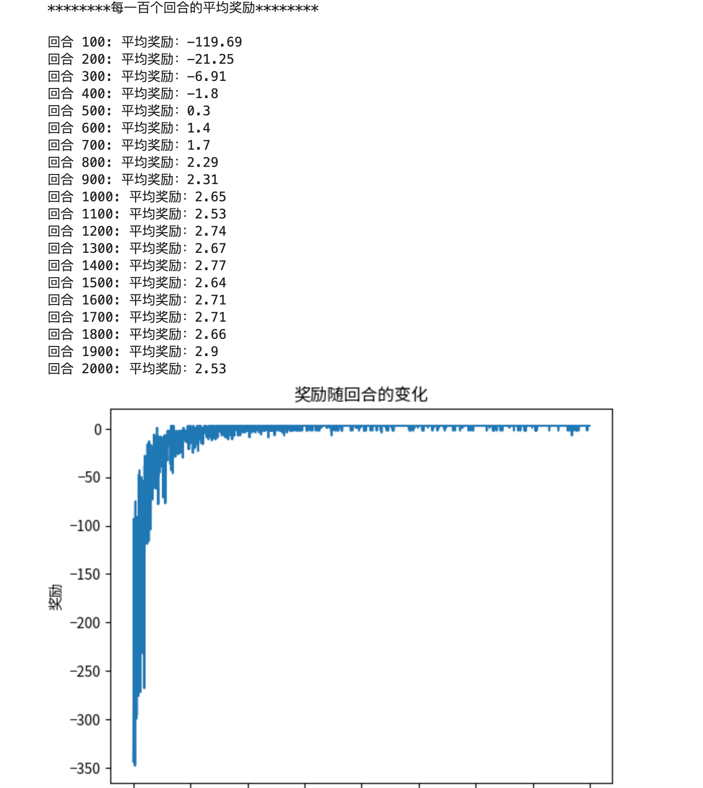
We can plot the cumulative reward of each training episode to watch the agent’s learning progress.

import matplotlib.pyplot as plt

# Average reward over every hundred episodes
rewards_per_hundred_episodes = np.split(np.array(rewards_all_episodes), num_episodes/100)

count = 100
print("********Average reward per hundred episodes********\n")
for r in rewards_per_hundred_episodes:
    print(f"Episode {count}: average reward: {sum(r)/100}")
    count += 100

# Plot the reward curve
plt.plot(rewards_all_episodes)
plt.xlabel('Episode')
plt.ylabel('Reward')
plt.title('Reward over episodes')
plt.show()

Sample output:

That covers everything in this chapter.